Query Data with SQL

A SQL cell runs a query and leaves the answer in the kernel as a pandas DataFrame, for the Python cells after it. This tutorial builds a database of every yellow taxi trip in New York in January 2024, about three million of them, connects Zasper to it, and asks it which boroughs the trips start in and what they cost.

You need a Python kernel with pandas in it. Your First Notebook covers getting one.

Get the Data

New York’s Taxi and Limousine Commission publishes every trip as a Parquet file. Make a notebook at the root of your project. The build reads the Parquet file with DuckDB, so install it first, in a cell of its own:

%pip install duckdb

Then run this. It downloads January 2024 and the list of taxi zones, and writes them to data/nyc_taxi.db, a SQLite database of about 400 MB:

import csv, io, os, sqlite3, urllib.request

import duckdb

TLC = "https://d37ci6vzurychx.cloudfront.net"
os.makedirs("data", exist_ok=True)
urllib.request.urlretrieve(f"{TLC}/trip-data/yellow_tripdata_2024-01.parquet", "data/yellow_2024-01.parquet")
with urllib.request.urlopen(f"{TLC}/misc/taxi_zone_lookup.csv") as response:
    zones = list(csv.reader(io.TextIOWrapper(response)))[1:]

db = sqlite3.connect("data/nyc_taxi.db")
db.executescript("""
CREATE TABLE zones (location_id INTEGER PRIMARY KEY, borough TEXT, zone TEXT, service_zone TEXT);
CREATE TABLE payment_types (payment_type INTEGER PRIMARY KEY, name TEXT);
CREATE TABLE trips (
  vendor_id INTEGER, pickup_at TEXT, dropoff_at TEXT, passenger_count INTEGER, trip_distance REAL,
  rate_code_id INTEGER, store_and_fwd_flag TEXT, pickup_location_id INTEGER, dropoff_location_id INTEGER,
  payment_type INTEGER, fare_amount REAL, extra REAL, mta_tax REAL, tip_amount REAL, tolls_amount REAL,
  improvement_surcharge REAL, total_amount REAL, congestion_surcharge REAL, airport_fee REAL);
INSERT INTO payment_types VALUES (0, 'Flex fare'), (1, 'Credit card'), (2, 'Cash'), (3, 'No charge'),
  (4, 'Dispute'), (5, 'Unknown'), (6, 'Voided trip');
""")
db.executemany("INSERT INTO zones VALUES (?, ?, ?, ?)", zones)
trips = duckdb.sql("""
  SELECT VendorID, strftime(tpep_pickup_datetime, '%Y-%m-%d %H:%M:%S'),
         strftime(tpep_dropoff_datetime, '%Y-%m-%d %H:%M:%S'), passenger_count, trip_distance,
         RatecodeID, store_and_fwd_flag, PULocationID, DOLocationID, payment_type, fare_amount, extra,
         mta_tax, tip_amount, tolls_amount, improvement_surcharge, total_amount, congestion_surcharge,
         Airport_fee
  FROM 'data/yellow_2024-01.parquet'
  WHERE tpep_pickup_datetime >= '2024-01-01' AND tpep_pickup_datetime < '2024-02-01'
  ORDER BY tpep_pickup_datetime""")
while batch := trips.fetchmany(200_000):
    db.executemany(f"INSERT INTO trips VALUES ({', '.join('?' * 19)})", batch)
db.execute("CREATE INDEX trips_pickup_at ON trips (pickup_at)")
db.commit()
db.close()
os.remove("data/yellow_2024-01.parquet")

It takes a few minutes, most of them downloading. The database has three tables:

Add a Connection

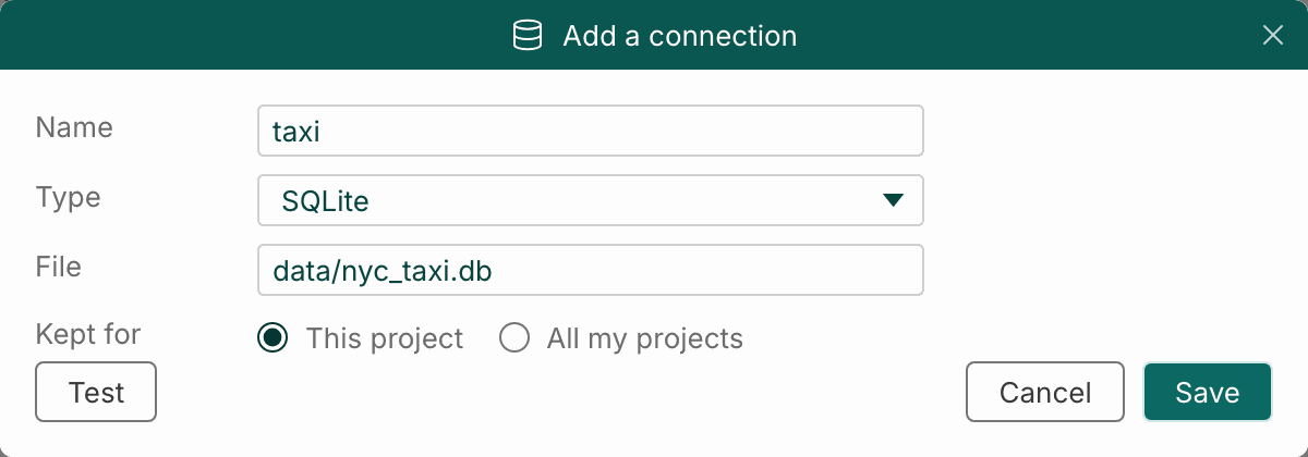
Open Settings from the gear in the sidebar, go to Data connections, and press Add…. Fill in:

• Name: taxi. A SQL cell names the connection it runs on by this.
• Type: SQLite.
• File: data/nyc_taxi.db. A path that is not absolute is read from the project’s root.
• Kept for: This project, so the connection is saved in the project’s .zasper/connections.json and can be committed with it. SQLite has no password. For a database that does, the password goes into your system keychain, never into that file.

Test opens the database and says how quickly it answered. Then Save.

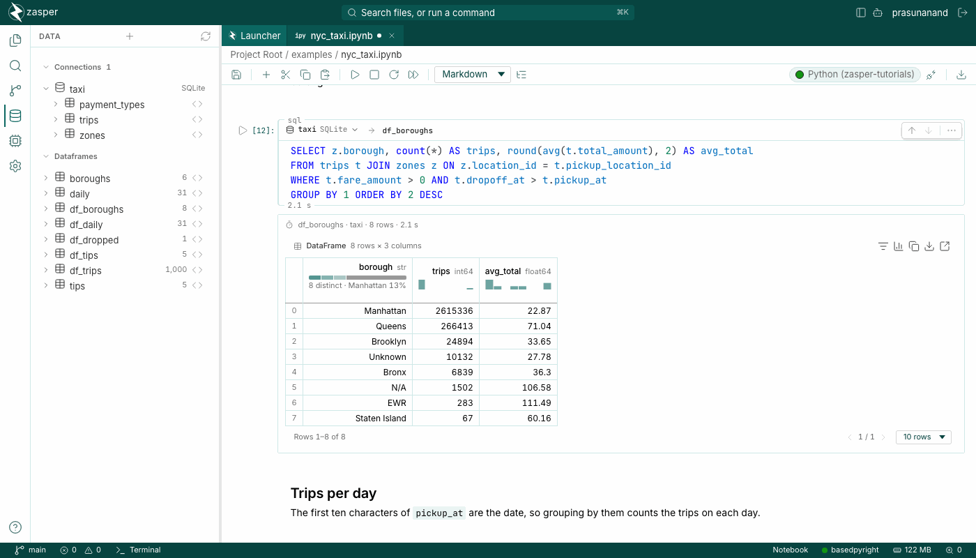
Data in the sidebar now lists taxi. Open it to see its tables, and a table to see its columns and their types.

Ask a Question

Point at the gap below the cell you ran, and choose SQL on the rail that appears. The new cell’s head says where it runs and where the answer goes: on taxi, the project’s first connection, into df_1. Click df_1 and rename it df_boroughs. Then type the query, and run it with Shift+Enter:

SELECT z.borough, count(*) AS trips, round(avg(t.total_amount), 2) AS avg_total
FROM trips t JOIN zones z ON z.location_id = t.pickup_location_id
WHERE t.fare_amount > 0 AND t.dropoff_at > t.pickup_at
GROUP BY 1 ORDER BY 2 DESC

As you type, the editor completes table and column names from the database. The WHERE line leaves out refunds and corrections, which are recorded as trips with a negative fare, and trips that end before they start.

The query runs in the database, over all three million trips, and brings back only its eight rows. The output’s first line names the DataFrame and the connection, counts the rows and says how long the query took. The rows follow as a table you can page, sort, filter and chart.

More Rows Than It Shows

Now ask for every trip, in a SQL cell of its own:

SELECT * FROM trips

A SQL cell reads at most 1,000 rows unless told otherwise, and says when it left rows behind. Press Load all once, and it counts them and estimates the memory reading them would take:

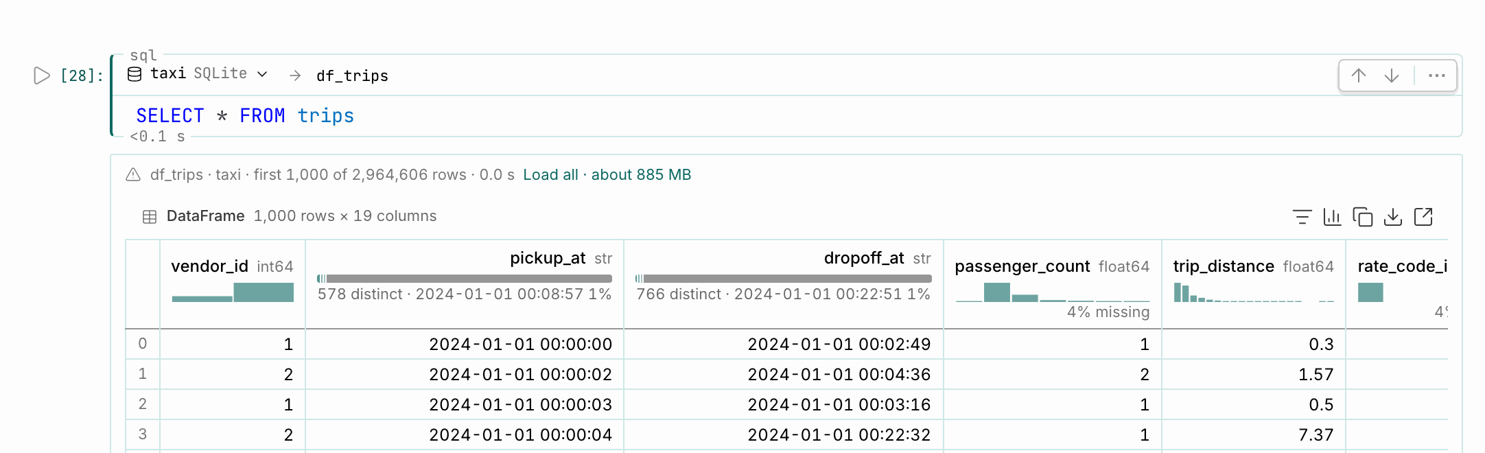
Pressing it again reads all 2,964,606 rows. Usually you do not want to: a query that groups, counts or averages in the database, like the one before it, brings back the answer rather than the rows.

Use the Answer in Python

df_boroughs is an ordinary DataFrame. In a code cell below it:

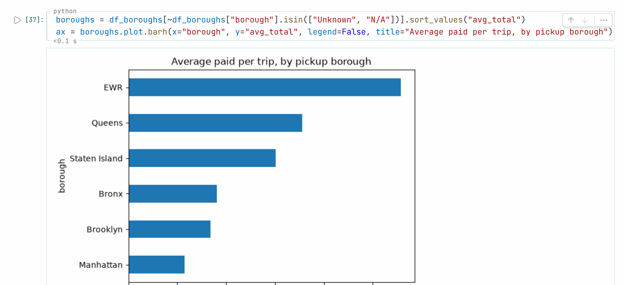
boroughs = df_boroughs[~df_boroughs["borough"].isin(["Unknown", "N/A"])].sort_values("avg_total")
ax = boroughs.plot.barh(x="borough", y="avg_total", legend=False, title="Average paid per trip, by pickup borough")

Unknown and N/A are zones with no borough. The language server knows df_boroughs too, so it is not flagged as undefined, and df_boroughs. completes as a DataFrame.

In the Notebook File

A SQL cell is saved as a code cell whose first line is a cell magic, so the notebook stays an ordinary .ipynb:

%%zasper_sql taxi --out df_boroughs
SELECT z.borough, count(*) AS trips, round(avg(t.total_amount), 2) AS avg_total
...

Zasper hides that line and shows the cell’s head instead. JupyterLab does not know the magic, so the cell runs only in Zasper.

SQL Cells has the rest: PostgreSQL, MySQL, Snowflake and the other databases, querying the kernel’s own DataFrames with DuckDB, the answer cache, and the Data panel.